Check Multiple Criteria with Excel INDEX and MATCH

Article from: http://blog.contextures.com/archives/2012/07/12/check-multiple-criteria-with-excel-index-and-match/

The INDEX function can return a value from a range of cells, and the MATCH function can calculate a value's position in a range of cells.

For example, in the screen shot below, cell A7 contains the item name, Sweater:

• the MATCH function can find "Sweater" in the range B2:B4. The result is 1, because "Sweater" is in the first row of that range.
• the INDEX function can tell you that in the range C2:C4, the first row contains the value 10.

So, by combining INDEX and MATCH, you can find the row with "Sweater" and return the price from that row.

=INDEX($C$2:$C$4,MATCH(A7,$B$2:$B$4,0))

Find a Match for Multiple Criteria

In the previous example, the match was based solely on the Item name – Sweater. Sometimes life, and Excel workbooks, are more complicated.

In the screen shot below, each item is listed 3 times in the pricing lookup table. To get the right price, you'll need to specify both the item name and the size. We want to find the price for a large jacket.

Does it MATCH? True or False

Instead of a simple MATCH formula, we'll use one that checks both the Item and Size columns. To do something similar on a worksheet, we could add columns to check the item and size columns.

• If the Item in column B is a Jacket, the result in column E is TRUE. If not, the result is FALSE
• If the Size in column C is Large, the result in column F is TRUE. If not, the result is FALSE

In column G, when you multiply the TRUE/FALSE values, the result is 1, only if both are TRUE.

We could use a MATCH formula to find the position of a 1 in column G, in the screen shot above. The 8th row of data (worksheet row 9), has the 1, and that row will give us the correct price for a large jacket.

Use MATCH With Multiple Criteria

Instead of adding extra columns to the worksheet, we can use an array-entered formula to do all the work. Here is the formula that we'll use to get the correct price, and below is the explanation:

=INDEX($D$2:$D$10,
MATCH(1,(A13=$B$2:$B$10)*(B13=$C$2:$C$10),0))

NOTE: This is an array-entered formula, so press Ctrl + Shift + Enter, instead of just pressing the Enter key.

In this example,

• prices are in cells D2:D10, so that is the range that the INDEX function will use.
• item name is in cell A13
• size is in cell B13.

The formula checks for the selected items in $B$2:$B$10, and sizes in $C$2:$C$10. The results are multiplied.

• (A13=$B$2:$B$10)*(B13=$C$2:$C$10)

The MATCH function looks for the 1 in the array of results.

• MATCH(1,(A13=$B$2:$B$10)*(B13=$C$2:$C$10),0)

If you select that part of the formula and press the F9 key, you can see the calculated results. In the screen shot below there are 9 results, and all are zero, except the 8th result, which is 1.

So, the INDEX function returns the price – 40 – from the 8th data row in column D (cell D9).

To find the product code for the selected item and size, you would change the formula to look in cells A2:A10, instead of the price column.

=INDEX($A$2:$A$10,
MATCH(1,(A13=$B$2:$B$10)*(B13=$C$2:$C$10),0))

In this example, the product code would be JK003, from cell A9.

Excel Formula: Compare Column A and B in Sheet1 and Sheet2, If matches copy Column C and Column D data from Sheet1 to Sheet 2

Compare Sheet1.Column A with Sheet2.Column A, If matches then compare Sheet1.Column B with Sheet2.Column B. If matches copy Sheet1.Column C and Sheet1.Column D data to Sheet2.Column E and Sheet2.Column G.

Sheet1




Sheet2


Result


Formula: 
=IF(AND(COUNTIF(Sheet2!A2,Sheet1!A2),(COUNTIF(Sheet2!B2,Sheet1!B2))),Sheet1!C2,0)

Compare Two or More Lists in Excel with IF and COUNTIF

Article from: http://www.bighungrygeek.com/compare-two-or-more-lists-in-excel-with-if-and-countif

As I previously discussed, Excel provides many useful ways to automatically compare two lists of data or information. In our other example we compared two lists of four digit account values; for this example we’ll compare two lists of names.

You and a friend are throwing an epic party and have each maintained separate guest lists to track who’s coming. After a few weeks you decide to compare both lists to make sure everyone on your friend’s list (List B) is also on your list (List A).

How to do it

1. Arrange the lists in two columns with List A in column A and List B in column B.
2. Create a third column in column D called List C (leave column C blank for easier readability).
3. In cell D5 enter the formula: =IF(COUNTIF(B:B,A5),A5,0) and press Enter.
   
   

   Enter formula into cell D5.
4. Select cell D5 and navigate to Home → Conditional Formatting → Highlight Cell Rules → Equal To…
5. In the Equal To dialog box, type 0 and click OK.
6. Select cell D5 down to the end of the lists and press Ctrl+D to copy the formula and conditional formatting down.
   
   

   Copy the formula down to the end of the lists.

The Result

A name in List C means the corresponding name from List A was also found within List B. In the screenshot above, cell D5 displays the “Moon Barrientos,” which means that name was found on both List A and B. On the other hand, cell D12 displays  which means the corresponding name from List A (in this case, “Aracely Rock”) does not exist within List B.

This example demonstrates how to determine if a particular value – in this case a name – in List A also exists within List B. To find the opposite – whether a name in List B also exists within List A – simply change the formula in cell D5 to: =IF(COUNTIF(A:A,B5),B5,0) and press Enter. Then copy that formula down to the end of the lists.

How & Why it Works

Our formula makes use of two functions, IF and COUNTIF. The IF function checks whether a condition is met, and returns one value if TRUE, and another value if FALSE. COUNTIF counts the number of cells within a range that meet the given condition.

The Formula

=IF(COUNTIF(B:B,A5),A5,0)

COUNTIF has two required arguments, or inputs, to work:

• range (where should Excel look, B:B in our example)
• criteria (what should Excel find, A5 in our example)

COUNTIF checks column B (using B:B checks the entire column) for the name in cell A5. If it finds the name (i.e. the criteria you specified was met) it returns 1, otherwise it returns 0. Note: whenCOUNTIF returns 1 or 0, Excel treats that as TRUE (1) or FALSE (0).

The IF function has three required arguments, or inputs, to work:

• logical_test (any value or expression that can be evaluated to TRUE or FALSE)
• [value_if_true] (what value should Excel return if if logical_test is TRUE)
• [value_if_false] (what value should Excel return if logical_test is FALSE)

In our example COUNTIF is the logical_test that gives the IF function either a 1 or 0, depending on whether it finds the name we specified from cell A5 within column B. If it finds the name (i.e. thelogical_test is TRUE), we specified A5 as the [value_if_true] so Excel will display that name and move on. If it does not find the name (i.e. the logical_test is FALSE), we specified 0 as the[value_if_false], so Excel will display 0 and move on.

You can quickly see a list of names missing from List B by filtering List C to show only “0.” The conditional formatting just makes it easier to spot the missing values.

Find Duplicates and Triplicates in Excel

Source from:http://exceliseasy.wordpress.com/2012/11/12/find-duplicates-and-triplicates-in-excel/

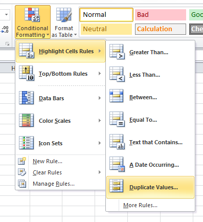
Select the cells you want to check and choose Highlight Cell Rules => Duplicate Values from the Home Ribbon.

Then, the easy way

If you only want to locate the duplicates, the super-easy way is the right way to do it. But let’s say you want to find triplicates or quadruplicates, i.e. three or four occurrences of the same piece of data. There is no built-in feature for that, so we have to find our own way.

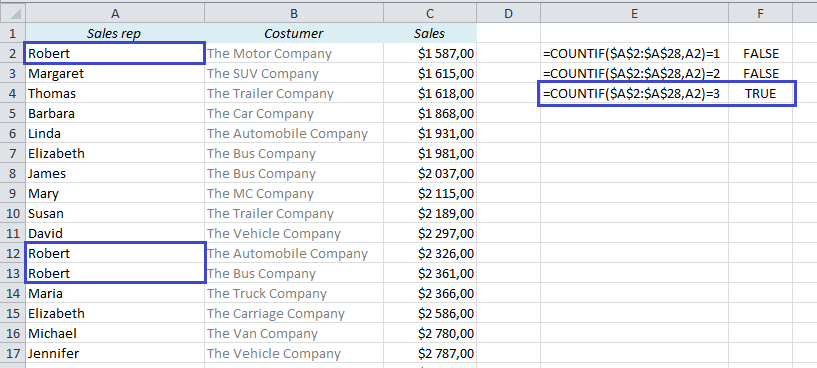
In my example I have 27 rows of data, with names in the range A2 to A28. In A2 we find the name Robert, so if we want to find out how many times Robert appears in the list, this is the formula: =COUNTIF($A$2:$A$28,A2). We’ll use Conditional Formatting with a formula like this.

As we’ve seen in a previous post, Conditional Formatting requires a TRUE or FALSE. Let’s see how our formula works when we put it in the worksheet. We use the same formula as above, only with “=1”, “=2” or “=3” in the end, and we will get TRUE or FALSE for each statement:

So, let’s put this formula into Conditional Formatting, with one small adjustment: Instead of hard-coding the value after the equal sign (1,2,3 etc.) we’ll use a cell reference. I will have my reference in cell E2.

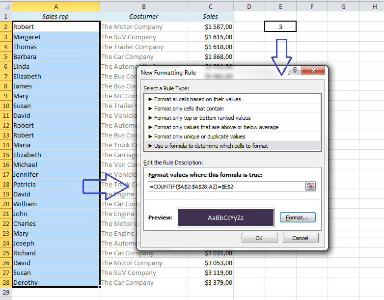
Select the cells you want to include in the search (A2:A28 in this example) and click on Conditional Formatting from the Home ribbon and choose New Rule (or shortcut: Alt => H => L => N). Choose “Use a formula to determine which cells to format” and type the formula into the formula field:

=COUNTIF($A$2:$A$28,A2)=$E$2

Note that the range A2:A28 and the reference to E2 (number of occurrences) have to be locked with dollar signs (shortcut: F4).

The result: All the triplicates are highlighted. If you change the value in E2 to 2, you will get the duplicates instead, and if you change it to 1, only the unique values will be highlighted.

Extra: Do you want to learn how to create a search field in your Excel report? Have a look at this post (opens in new window/tab): Create a search field in Excel in 5 minutes

Note: If you use comma as the decimal separator as default (applies to most non-English users) you have to replace the commas in the formulas with semicolons.

Excel: IF

1 2 3 4 5 6 7 8

A B C Score 45 90 78 Formula Description Result =IF(A2>89,"A",IF(A2>79,"B", IF(A2>69,"C",IF(A2>59,"D","F")))) Assigns a letter grade to the score in cell A2 F =IF(A3>89,"A",IF(A3>79,"B", IF(A3>69,"C",IF(A3>59,"D","F")))) Assigns a letter grade to the score in cell A3 A =IF(A4>89,"A",IF(A4>79,"B", IF(A4>69,"C",IF(A4>59,"D","F")))) Assigns a letter grade to the score in cell A4 C

Excel : SEARCH and FIND

Source from: http://www.myonlinetraininghub.com/excel-search-and-you-will-find

IF(ISNUMBER(SEARCH("brown",A20)),$F$20,$F$21)

1. Convert the result to a TRUE/FALSE answer using ISNUMBER and then use it in an IF statement to return a value for ‘brown foxes’ and a different value for everything else.


Brief Explanation: The formula in cell B20 is searching for the word ‘brown’, if the result is a number (ISNUMBER) then choose the value in cell F20, and if it’s not (if the word isn’t found SEARCH will return a #N/A error) then choose the value in cell F21.



1. Use it as an array formula to count the number of instances of a word occurring in text strings in a range of cells.

Note: the formula is entered =COUNT(IF(SEARCH(“brown”,A32:A35),1,”")) and then you press CTRL+SHIFT+ENTER to enter it as an array formula and Excel will enter the curly brackets for you.
If you liked this let me know by clicking the Facebook like, Tweet it or simply leave a comment below. I’d love to hear from you and how you use these functions.